Hello world

To follow this guide you only need to know what a Normal distribution is and what an integral is, by the end you will hopefully understand the Metropolis algorithm intuitively (the what, the why and the how), and learn about statistical modelling and Bayesian statistics along the way.

Introduction

Metropolis is a prince of an algorithm.

It's like a drunk person stumbling home, and as they wander erratically in a homeward direction they come to understand a complex problem beyond the capability of a cogent scholar.

And it's the wandering, the erratic path, that can solve the impossible.

A glimpse

To see the Metropolis algorithm in action, try this interactive simulator.

The yellow square is some unknown part of reality, an entity or process floating in probability space. The entity has three attributes, each represented by an axis in the 3D space. In a real world setting, the location of the yellow square (the values of its attributes) would be unknown to us. All we have are some scattered, noisy observations.

The cyan circle is our starting point, representing our initial hypothesis about the value of each attribute.

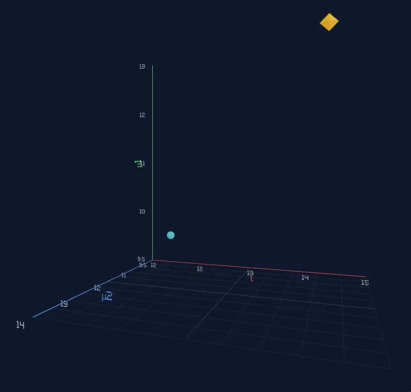
Press the Full Auto button in the sidebar and watch the algorithm locate the yellow square. You can rotate, pan and zoom using your mouse controls / trackpad / touch. Press Reset and then press Full Auto a few more times. Observe that the algorithm takes a different trajectory every time. It’s a homing missile that finds the target and encloses it within its probability cloud (posterior distribution).

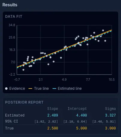
The Results section shows this plot. The yellow line is the actual entity that we're trying to capture, in this experiment it's a linear process. Around the yellow line are white dots representing individual observations of the process. The three attributes are: the slope of the line, the y-axis intercept of the line, and the noise (standard deviation) of the observations.

The cyan dashed line is our best estimate of the yellow line based on the probability cloud (posterior distribution). Click Reset and Full Auto again and watch the cyan line converge upon the yellow line as the algorithm progresses.

The Posterior Report underneath contains our best estimates of the attributes and our uncertainty about them (95% credible intervals), as well as their true values.

We don't want the 'contrails' to form part of our final belief, so we usually ignore the first N number of steps. Change the Burn-in setting in the sidebar to a value of 70 and press Full Auto again.

To understand how the algorithm works, we’re going to look at a more interesting problem.

A problem

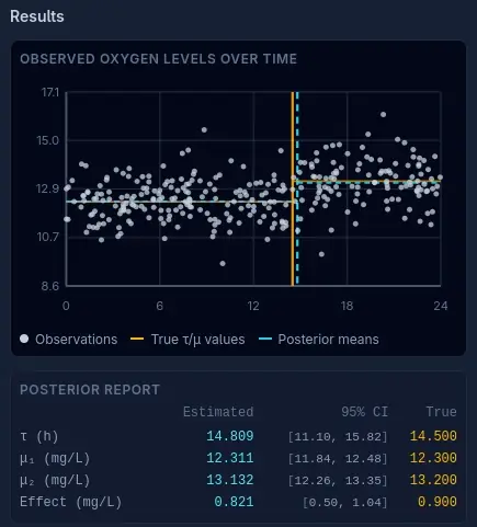
Suppose that we are monitoring the levels of dissolved oxygen (mg/L) in stream water. Samples collected at random times over a 24 hour period suggest that there was a change-point in the early afternoon:

We want to find out:

when did the change-point most likely occur, and a credible interval (Bayesian equivalent of a confidence interval)
what was the most likely magnitude of the change, and a credible interval

We're going to construct a Bayesian model for the data:

a Bayesian model allows us to answer questions like "what is the probability that the change-point occurred between 4:40pm and 4:50pm?"
Bayesian approaches can provide a more complete understanding of complex (high dimensional) problems
Bayesian modelling is a common use case for the Metropolis algorithm

The model

We propose a model for the oxygen level consisting of the unknown change-point time $\tau$ in fractional hours (e.g. 14.5 is 2:30pm) and two normal distributions of oxygen levels (mg/L) with unknown means $\mu_1$ (the mean oxygen level before $\tau$) and $\mu_2$ (the mean oxygen level after $\tau$). Each unknown attribute of the underlying reality $\tau$, $\mu_1$, $\mu_2$, is a model parameter. For the sake of keeping the model parameters within 3 dimensions, the real standard deviation $\sigma$ of oxygen levels is a known constant of +/- 0.9 mg/L. The model of oxygen level $l$ at time $t$ can be expressed as:

$$l_t \sim \begin{cases} \operatorname{Normal}(\mu_1, 0.9^2) & \text{if } t < \tau \\ \operatorname{Normal}(\mu_2, 0.9^2) & \text{if } t \ge \tau \end{cases}$$

There exists some time τ where the mean oxygen level shifted. Before τ, observations come from $\operatorname{Normal}(\mu_1, 0.9^2)$. After τ, they come from $\operatorname{Normal}(\mu_2, 0.9^2)$.

The challenge is to estimate $\tau$, $\mu_1$ and $\mu_2$ given the data, ideally we would like to do this using Bayes Theorem.

Note

We assume that the model is true, the challenge is to find the correct values of the parameters. For the purpose of our example the model will actually be true — the process which generates the observed data will indeed be two Normal distributions and a change point. In a real world situation we might want to compare our model against other models, including a model which has no change point (the null hypothesis). Instead of claiming that models are true or false, we say that there are models which are better or worse at describing and predicting reality.

A new simulator

Have a go with this simulator for our change-point model.

The Results section shows a plot of the observational data and the real and estimated values of $\tau$, $\mu_1$, $\mu_2$ and the effect size ($\mu_2 - \mu_1$).

Bayes Theorem

The data is constant and known. The real values of $\tau, \mu_1$ and $\mu_2$ are unknown, we will vary their hypothetical values and calculate the probability of each combination to build a probability distribution for all possible hypotheses. Each unique combination of values for $\tau, \mu_1$ and $\mu_2$ forms a hypothesis $\theta_i$ in the set of hypotheses under consideration $\theta$. This will allow us to find the most likely hypothesis (the most likely values of $\tau, \mu_1$ and $\mu_2$.)

Bayes Theorem relates three functions that depend on $\theta$ and a constant factor that involves the data alone.

$$p(\theta \mid \text{data}) = \frac{p(\text{data} \mid \theta) \cdot p(\theta)}{p(\text{data})}$$

$p(\theta \mid \text{data})$ the posterior distribution — the probability distribution of hypotheses $\theta$ given (conditional on) the data — this is what we want to obtain.

$p(\text{data} \mid \theta)$ the likelihood function — the likelihood of observing the data conditional on a given hypothesis $\theta$.

Likelihood versus probability

If we held the hypothesis $\theta$ constant and calculated $p(\text{data} \mid \theta)$ for all possible $\text{data}$ sets then $p(\text{data} \mid \theta)$ would be a probability distribution because the integral over $\text{data}$ would always be equal to 1. But because we are holding $\text{data}$ constant and the integral over $\theta$ does not always equal 1, $p(\text{data} \mid \theta)$ expresses a likelihood (a score) not a probability, this is why we call it a likelihood function and not a probability distribution.

We can use ratios of likelihoods to express the probability of one outcome relative to another, but not their absolute probabilities.

$p(\theta)$ the prior distribution — the probability distribution of hypotheses $\theta$ given our beliefs before seeing the data. Imagine that we haven't seen the data, in our state of ignorance what would our beliefs about time $\tau$ and the means $\mu_1$ and $\mu_2$ be? We need to express those beliefs as a probability distribution.

$p(\text{data})$ the evidence — how probable is the data in general regardless of which hypothesis is true? $p(\text{data})$ is calculated by integrating the probability of observing the data given a hypothesis weighted by the probability of the given hypothesis itself.

$$p(\mathrm{data}) = \int p(\mathrm{data}\mid \theta) \cdot p(\theta)\, d\theta$$

This is the constant, normalisation factor which turns the product of the likelihood function and the prior probability distribution from being a likelihood ratio into the posterior probability distribution.

Bayes Theorem restated — Given the data, the probability of a hypothesis equals how likely the observed data would be if the hypothesis were true, multiplied by the plausibility of the hypothesis in general (without seeing the data), divided by how likely the observed data is overall (regardless of which hypothesis is true.)

Practical limitations on using Bayes Theorem

The integral for the evidence $p(\text{data})$ is often a stumbling block.

Ideally we would like to compute the exact values of integrals by deriving their analytical, closed-form solutions:

$$ \int x^2 \, dx = \frac{1}3x^3 + C \\ \int_{2}^{5} x^2 \, dx = (\frac{1}3 \cdot 5^3 + C) - (\frac{1}3 \cdot 2^3 + C) = 39 $$

When finding a closed-form solution is analytically intractable we can use numerical integration to find an inexact solution. The above example could be solved by computing “the area under the curve”:

$$\int_{2}^{5} x^{2}\,dx \approx \sum_{i=1}^{n} f(x_i^{*})\,\Delta x$$

We would like an analytical solution for $p(\text{data})$:

$$p(\mathrm{data}) = \int p(\mathrm{data}\mid \theta) \cdot p(\theta)\, d\theta$$

In our model this is a three-dimensional integral:

$$p(\mathrm{data}) \;=\; \iiint p(\mathrm{data}\mid \tau,\mu_1,\mu_2)\, p(\tau)\, p(\mu_1)\, p(\mu_2)\, d\tau\, d\mu_1\, d\mu_2$$

For our simple model, this is in fact analytically tractable. Very often it isn't. For example, we could (but we won't) acknowledge that negative oxygen levels are not physically possible and represent that condition in our model by using a LogNormal instead of a Normal distribution. That minor change would make $p(\text{data})$ analytically intractable.

If we did do that, we might then use numerical integration (quadrature): 1) we split the 3-dimensional space into a grid of many small blocks, 2) we calculate $p(\mathrm{data}\mid \tau,\mu_1,\mu_2)\, p(\tau)\, p(\mu_1)\, p(\mu_2)$ by plugging in the values of $\tau$, $\mu_1$ and $\mu_2$ for each grid block and multiplying by the block volume, and 3) we sum the calculations over all grid blocks.

With just three dimensions (parameters) that is also easily doable.

Numerical integration rapidly becomes infeasible as the number of parameters increases, typically beyond 5–10 parameters. Numerically integrating over 7 parameters with a low grid resolution of 20 points per parameter is 1.3 billion computations. Increase that to 10 parameters and it becomes 10 trillion computations.

Another limitation is that numerical integration struggles to accurately represent a complex posterior distribution (e.g. skewed, many modes).

When $p(\text{data})$ is analytically intractable and numerical computation is too expensive or the posterior distribution is too complex, an alternative is to use a Markov chain Monte Carlo method like the Metropolis algorithm.

The Metropolis algorithm

The posterior odds

Recall Bayes Theorem:

$$p(\theta \mid \text{data}) = \frac{p(\text{data} \mid \theta) \cdot p(\theta)}{p(\text{data})}$$

If we divide Bayes theorem for any hypothesis $\theta_2$ by Bayes theorem for any other hypothesis $\theta_1$ the normalisation factor $p(\text{data})$ cancels out:

$$\begin{aligned} \frac{p(\theta_2\mid \text{data})}{p(\theta_1\mid \text{data})} &=\frac{p(\text{data} \mid \theta_2) \cdot p(\theta_2)}{p(\text{data})} \cdot\frac{p(\text{data})}{p(\text{data} \mid \theta_1) \cdot p(\theta_1)} \\ \\ &= \frac{p(\text{data}\mid \theta_2)}{p(\text{data}\mid \theta_1)} \cdot \frac{p(\theta_2)}{p(\theta_1)} \end{aligned}$$

Some new terminology:

$$\underbrace{\frac{p(\theta_2\mid \text{data})}{p(\theta_1\mid \text{data})}}_{\text{posterior odds}}=\underbrace{\frac{p(\text{data}\mid \theta_2)}{p(\text{data}\mid \theta_1)}}_{\text{likelihood ratio}}\cdot\underbrace{\frac{p(\theta_2)}{p(\theta_1)}}_{\text{prior odds}}$$

The posterior odds is the ratio of how much more likely one hypothesis is versus another (the ratio of their posterior probability densities). We can calculate this without ever needing to calculate the normalisation factor $p(\text{data})$.

The likelihood ratio is a measure of how strongly the evidence supports one hypothesis versus another.

The prior odds is how much more feasible one hypothesis is versus another in general, it's our prior belief without seeing the data.

The algorithm

Select an initial current hypothesis $\theta_\text{current}$ by choosing values for parameters $\tau$, $\mu_1$ and $\mu_2$ anywhere in the model probability space (this initial starting position is often informed by the data).
Propose a new hypothesis $\theta_\text{proposal}$: select new values for the parameters $\tau$, $\mu_1$ and $\mu_2$ by picking a random value within a defined range (a proposal width) around each of the existing values for $\tau$, $\mu_1$ and $\mu_2$ in $\theta_\text{current}$.
Calculate the posterior odds for $\theta_\text{proposal}$ over $\theta_\text{current}$.
$$\frac{p(\theta_\text{proposal}\mid \text{data})}{p(\theta_\text{current}\mid \text{data})}=\frac{p(\text{data}\mid \theta_\text{proposal})}{p(\text{data}\mid \theta_\text{current})}\cdot\frac{p(\theta_\text{proposal})}{p(\theta_\text{current})}$$
In this step we choose to accept either $\theta_\text{proposal}$ or $\theta_\text{current}$ as hypothesis $\theta_\text{accepted}$:
- If $\theta_\text{proposal}$ is more likely than $\theta_\text{current}$ (posterior odds ≥ 1) then $\theta_\text{accepted}=\theta_\text{proposal}$
- If $\theta_\text{proposal}$ is less likely (posterior odds < 1), we use a random number generator to accept one of the hypotheses by chance. The probability of accepting $\theta_\text{proposal}$ is set to the posterior odds and therefore the probability of accepting $\theta_\text{current}$ is 100% − the posterior odds (in practise we'll be using fractional probabilities, so 1 - the posterior odds).
  
  E.g. if the posterior odds = 0.8:
  
  => set an 80% chance of selecting $\theta_\text{accepted} = \theta_\text{proposal}$
  
  => there's a 20% chance of selecting $\theta_\text{accepted} = \theta_\text{current}$
  
  This is the crucial part of the algorithm: even though $\theta_\text{proposal}$ is less likely (80% as likely as $\theta_\text{current}$), there's an 80% chance that we'll accept it anyway
Record $\theta_\text{accepted}$ (parameter values).
Jump back to step 2), set $\theta_\text{current}$ to the value of $\theta_\text{accepted}$ and create a new $\theta_\text{proposal}$.
Repeat this loop until there are enough (many!) records.

Each recorded hypothesis $\theta_\text{accepted}$ is a sample from an approximation to the posterior distribution and the samples converge to the true posterior distribution $p(\theta \mid \text{data})$ as the number of samples approaches infinity. This process allows us to construct the posterior distribution without ever knowing the $p(\text{data})$ normalisation factor.

It's the ability to jump to less likely locations in the hypothesis space (when the posterior odds < 1 and we accept $\theta_\text{proposal}$) that constructs the posterior distribution. If we always accepted the most likely hypothesis out of $\theta_\text{proposal}$ and $\theta_\text{current}$ we would create a speed running hill climb to the most likely hypothesis (mode) of the posterior distribution, and although this point value is of interest, the process wouldn't give us the posterior distribution itself as it wouldn't sample the full probability space — we would have the mode but no estimation of its uncertainty. A hill climb also has greater risk of getting stuck in a local maximum if the distribution has multiple modes, i.e. it wouldn't be able to map a multi modal distribution.

Markov chain Monte Carlo

You'll often see the Metropolis algorithm referred to as Markov chain Monte Carlo or MCMC for short.

A Markov chain is any sequence where the next state depends only on the current state, not on how you got there. At each step, we propose a move based on where we are now, evaluate whether to accept based on current versus proposed, and move (or stay). The entire history of where we've been is irrelevant to what happens next.

The "Monte Carlo" part refers to the randomness — we're using random sampling to explore the space by accepting/rejecting proposals.

Worked example for oxygen levels

We need to derive the posterior odds equation used in the proposal step:

$$\underbrace{\frac{p(\theta_{\text{proposal}}\mid \text{data})}{p(\theta_\text{current}\mid \text{data})}}_{\text{posterior odds}}=\underbrace{\frac{p(\text{data}\mid \theta_\text{proposal})}{p(\text{data}\mid \theta_\text{current})}}_{\text{likelihood ratio}}\cdot\underbrace{\frac{p(\theta_\text{proposal})}{p(\theta_\text{current})}}_{\text{prior odds}}$$

Natural logarithms

We will be taking the natural logarithm of the equation for the posterior odds.

Probabilistic computing often involves multiplying fractional probabilities many times over, and the result can get very small very fast — too small for the computer's representation of floating point numbers. For this reason, and because it often simplifies the mathematical representations, calculations are done in log space.

Logarithm rules

$$\log(a \cdot b) = \log(a) + \log(b) \\ \log(a / b) = \log(a) - \log(b)$$

Taking natural logs of both sides, the posterior odds equation becomes:

$$\begin{aligned} \ln p(\theta_\text{proposal} \mid \text{data}) - \ln p(\theta_\text{current} \mid \text{data}) &= \ln p(\text{data} \mid \theta_\text{proposal}) - \ln p(\text{data} \mid \theta_\text{current})\\\\ &+ \ln p(\theta_\text{proposal}) - \ln p(\theta_\text{current}) \end{aligned}$$

1) The prior odds

$$\frac{p(\theta_\text{proposal})}{p(\theta_\text{current})}$$

The prior odds is the ratio of the prior distribution function applied to each hypothesis.

$p(\theta)$ the prior distribution — the probability distribution of hypotheses $\theta$ given our beliefs before seeing the data.

What are our beliefs before seeing the data?

The time of the change-point $\tau$

We have no reason to believe that the change point occurring at time $\tau_1$ is more or less likely than any other time $\tau_2$. Therefore we will model our prior belief as all times being equally likely by using a continuous uniform distribution for $\tau$ where $N$ is the total number of hours in the data.

$$\tau \sim \operatorname{Uniform}(0, N)$$

The mean oxygen levels $\mu_1$ and $\mu_2$ before and after the change-point $\tau$

Prior to seeing the data we have no knowledge of the sign or the magnitude of the change, so we'll represent that state of ignorance by setting $\mu_1$ and $\mu_2$ to the same value.

For our belief about the most likely value of the mean we would draw from our experience, or general public knowledge, or historical data from the stream in question. For this experiment we'll set it to $\mu_1 = 15.0\text{ mg/L}$ and $\mu_2 = 15.0\text{ mg/L}$.

Our beliefs would also acknowledge that the values of $\mu$ would tail off the further we get from the most likely value. We have no reason to believe that the distribution is skewed, so we'll use a symmetrical distribution.

Under these conditions the Normal distribution would be a suitable representation of our prior beliefs. We'll choose a standard deviation of +/- 5.0 mg/L, this places our prior belief as being 95% confident that $\mu_1$ and $\mu_2$ are somewhere between 5.2 mg/L and 24.8 mg/L.

$$\mu_1 \sim \mathrm{Normal}(15.0, 5.0^2) \\ \mu_2 \sim \mathrm{Normal}(15.0, 5.0^2)$$

Putting it together

Now we can construct the prior distribution $p(\theta)$ for our model.

Because the parameters in our prior distribution are independent (what we believe about $\tau$ has no impact on what we believe about $\mu_1$ or $\mu_2$) the prior distribution can be expressed as the product of the prior distributions of each model parameter (the multiplication rule for independent probabilities):

$$p(\theta) = p(\tau) \cdot p(\mu_1) \cdot p(\mu_2)$$

$\tau$ is distributed uniformly over the time period of the data.

$$\tau \sim \operatorname{Uniform}(0, N) \\ p(\tau) = \frac{1}{24}$$

The mean oxygen levels are Normally distributed:

$$\mu_1 \sim \mathrm{Normal}(15.0, 5.0^2) \\ \mu_2 \sim \mathrm{Normal}(15.0, 5.0^2) \\ p(\mu)=\frac{1}{\sigma\sqrt{2\pi}}\cdot\exp\!\left(-\frac{(\mu-M)^2}{2\sigma^2}\right),\quad \sigma=5.0,\; M=15.0 \\ p(\mu_1)=\frac{1}{5.0\sqrt{2\pi}}\cdot\exp\!\left(-\frac{(\mu_1-15.0)^2}{2\cdot5.0^2}\right) \\ p(\mu_2)=\frac{1}{5.0\sqrt{2\pi}}\cdot\exp\!\left(-\frac{(\mu_2-15.0)^2}{2\cdot5.0^2}\right)$$

The prior distribution becomes:

$$\begin{aligned} p(\theta) &= p(\tau) \cdot p(\mu_1) \cdot p(\mu_2)\\\\ &=\frac{1}{24}\cdot\frac{1}{5.0^2\cdot{2\pi}}\cdot\exp\!\left(-\frac{(\mu_1-15.0)^2}{2\cdot5.0^2}\right)\cdot\exp\!\left(-\frac{(\mu_2-15.0)^2}{2\cdot5.0^2}\right) \end{aligned}$$

Now we can express the prior odds (the constant factor cancels out):

$$\frac{p(\theta_\text{proposal})}{p(\theta_\text{current})} = \frac{ \exp\!\left(-\frac{(\mu_1^{\text{proposal}}-15.0)^2}{2\cdot5.0^2}\right)\cdot\exp\!\left(-\frac{(\mu_2^{\text{proposal}}-15.0)^2}{2\cdot5.0^2}\right) }{ \exp\!\left(-\frac{(\mu_1^{\text{current}}-15.0)^2}{2\cdot5.0^2}\right)\cdot\exp\!\left(-\frac{(\mu_2^{\text{current}}-15.0)^2}{2\cdot5.0^2}\right) }$$

We want this in log form:

$$\begin{aligned} \ln \! \frac{p(\theta_\text{proposal})}{p(\theta_\text{current})} &= \ln p(\theta_\text{proposal}) - \ln p(\theta_\text{current}) \\\\ &= -\frac{(\mu_1^{\text{proposal}}-15.0)^2}{2\cdot5.0^2} -\frac{(\mu_2^{\text{proposal}}-15.0)^2}{2\cdot5.0^2} \\\\ &+\frac{(\mu_1^{\text{current}}-15.0)^2}{2\cdot5.0^2} +\frac{(\mu_2^{\text{current}}-15.0)^2}{2\cdot5.0^2} \end{aligned}$$

The above equation for the feasibility of one hypothesis versus another makes intuitive sense.

We stated that we have no reason to believe that any change-point time $\tau$ is more likely than another: $\tau$ doesn't appear in the equation.

We stated that we have no reason to believe that the pre- change-point mean $\mu_1$ is greater or less than the post- change-point mean $\mu_2$ so we set a ballpark guess of 15.0 mg/L for both. The feasibility of a hypothesis then depends only on how far its values of $\mu_1$ and $\mu_2$ are from 15.0 mg/L.

Note on the properties of natural logarithms

If the logarithm is negative then the prior odds is less than 1: the proposal hypothesis is less likely than the current hypothesis according to our prior beliefs.

If the logarithm is 0 or positive then the prior odds is greater than or equal to 1: the proposal hypothesis is at least as likely than the current hypothesis according to our prior beliefs..

$$\ln \! \frac{p(\theta_\text{proposal})}{p(\theta_\text{current})} \begin{cases} < 0, & 0 < \frac{p(\theta_\text{proposal})}{p(\theta_\text{current})} < 1,\\ = 0, & \frac{p(\theta_\text{proposal})}{p(\theta_\text{current})} = 1,\\ > 0, & \frac{p(\theta_\text{proposal})}{p(\theta_\text{current})} > 1. \end{cases}$$

The further away from 15.0 mg/L that the means for $\theta_\text{proposal}$ become, the less positive or more negative the right-hand side of the log-form equation becomes. This implies a smaller value for the prior odds in the left-hand side, expressing reduced belief in $\theta_\text{proposal}$ relative to $\theta_\text{current}$:

$$\frac{p(\theta_\text{proposal})}{p(\theta_\text{current})}$$

Equivalently, the further away from 15.0 mg/L that the $\theta_\text{current}$ means become, the less negative or the more positive the right-hand side of the equation and the larger the value of the prior odds, expressing increasing belief in $\theta_\text{proposal}$ versus $\theta_\text{current}$.

2) The likelihood ratio

$$\frac{p(\text{data}\mid \theta_\text{proposal})}{p(\text{data}\mid \theta_\text{current})}$$

The likelihood ratio is the ratio of the likelihood scores for our two hypotheses given the data: the likelihood function for our model applied to each hypothesis.

$p(\text{data} \mid \theta)$ the likelihood function — the likelihood of observing the data conditional on a given hypothesis $\theta$.

Our model for the data is that before $\tau$ the oxygen level follows a Normal distribution with mean $\mu_1$ and after $\tau$ it follows a Normal distribution with mean $\mu_2$.

Recall that we said for the purpose of this example, $\sigma$ is a constant and we know its true value of +/- 0.9 mg/L.

$$l_t \sim \begin{cases} \operatorname{Normal}(\mu_1, 0.9^2) & \text{if } t < \tau \\ \operatorname{Normal}(\mu_2, 0.9^2) & \text{if } t \ge \tau \end{cases}$$

$l_t$ is a continuous variable representing the oxygen level at any time $t$. We want the probability density for each observation $\text{data}_i$ at time $t_i$ given the model parameters $\tau$, $\mu_1$ and $\mu_2$, which is just the Normal probability density function:

$$f(\text{data}_i \mid \tau,\mu_1,\mu_2)= \begin{cases} \dfrac{1}{\sqrt{2\pi}\cdot0.9}\exp\!\left(-\dfrac{(\text{data}_i-\mu_1)^2}{2\cdot0.9^2}\right), & \text{if } t_i < \tau,\\[8pt] \dfrac{1}{\sqrt{2\pi}\cdot0.9}\exp\!\left(-\dfrac{(\text{data}_i-\mu_2)^2}{2\cdot0.9^2}\right), & \text{if } t_i \ge \tau. \end{cases}$$

The likelihood function then is the product of all the probability densities for the complete set of observations.

$$\begin{aligned} p(\text{data} \mid \theta^{(\tau, \mu_1, \mu_2)}) &= \prod_{i}f(\text{data}_i \mid \tau,\mu_1,\mu_2) \\ &=\prod_{i} \dfrac{1}{\sqrt{2\pi}\cdot0.9} \cdot \prod_{i:\,t_i<\tau} \exp\!\left(-\frac{(\text{data}_i-\mu_1)^2}{2\cdot0.9^2}\right)\cdot \prod_{i:\,t_i\ge\tau}\exp\!\left(-\frac{(\text{data}_i-\mu_2)^2}{2\cdot0.9^2}\right) \end{aligned}$$

Now we can express the likelihood ratio (the constant factor cancels out):

$$\frac{p(\text{data}\mid \theta_\text{proposal})} {p(\text{data}\mid \theta_\text{current})} = \frac { \prod_{i:\,t_i<\tau^\text{proposal}}\exp\!\left(-\frac{(\text{data}_i-\mu_1^\text{proposal})^2}{2\cdot0.9^2}\right)\cdot \prod_{i:\,t_i\ge\tau^\text{proposal}}\exp\!\left(-\frac{(\text{data}_i-\mu_2^\text{proposal})^2}{2\cdot0.9^2}\right) }{ \prod_{i:\,t_i<\tau^\text{current}}\exp\!\left(-\frac{(\text{data}_i-\mu_1^\text{current})^2}{2\cdot0.9^2}\right)\cdot \prod_{i:\,t_i\ge\tau^\text{current}}\exp\!\left(-\frac{(\text{data}_i-\mu_2^\text{current})^2}{2\cdot0.9^2}\right) }$$

We take logs of both sides:

$$\begin{aligned} \ln \! \left( \frac {p(\text{data}\mid \theta_\text{proposal})} {p(\text{data}\mid \theta_\text{current})} \right) &= \sum_{i:\,t_i<\tau^\text{current}} \! \frac{(\text{data}_i-\mu_1^{(\text{current})})^2} {2\cdot0.9^2} + \sum_{i:\,t_i\ge\tau^\text{current}} \! \frac{(\text{data}_i-\mu_2^{(\text{current})})^2} {2\cdot0.9^2} \\\\ &- \sum_{i:\,t_i<\tau^\text{proposal}} \! \frac{(\text{data}_i-\mu_1^{(\text{proposal})})^2} {2\cdot0.9^2} - \sum_{i:\,t_i\ge\tau^\text{proposal}} \! \frac{(\text{data}_i-\mu_2^{(\text{proposal})})^2} {2\cdot0.9^2} \end{aligned}$$

This result again makes intuitive sense. Recall that for the prior odds ratio, the further that our proposed mean $\mu_1^{(\text{proposal})}$ was from our prior beliefs, the smaller the odds ratio expressing reduced belief in $\theta_\text{proposal}$. A similar thing is happening here for our likelihood ratio, except that this time it's the distance of $\mu_1^{(\text{proposal})}$ from the $\text{data}$.

3) The posterior odds

Now we have everything we need to calculate the posterior odds used in step 3) of the algorithm.

Taking logs:

Substituting our log form expressions for the likelihood ratio and the prior odds:

$$\begin{aligned} \ln p(\theta_\text{proposal} \mid \text{data}) - \ln p(\theta_\text{current} \mid \text{data}) &= \sum_{i:\,t_i<\tau^\text{current}} \! \frac{(\text{data}_i-\mu_1^{(\text{current})})^2} {2\cdot0.9^2} + \sum_{i:\,t_i\ge\tau^\text{current}} \! \frac{(\text{data}_i-\mu_2^{(\text{current})})^2} {2\cdot0.9^2} \\\\ &- \sum_{i:\,t_i<\tau^\text{proposal}} \! \frac{(\text{data}_i-\mu_1^{(\text{proposal})})^2} {2\cdot0.9^2} - \sum_{i:\,t_i\ge\tau^\text{proposal}} \! \frac{(\text{data}_i-\mu_2^{(\text{proposal})})^2} {2\cdot0.9^2} \\\\ &+\frac{(\mu_1^{\text{current}}-15.0)^2}{2\cdot5.0^2} +\frac{(\mu_2^{\text{current}}-15.0)^2}{2\cdot5.0^2} \\\\ &-\frac{(\mu_1^{\text{proposal}}-15.0)^2}{2\cdot5.0^2} -\frac{(\mu_2^{\text{proposal}}-15.0)^2}{2\cdot5.0^2} \end{aligned}$$

The algorithm revisited

Now we know how to compute the posterior odds we can run the algorithm. Recall the process:

Choose an initial hypothesis for $\theta_\text{current}$ anywhere in the parameter space, e.g.
- $\mu_1^\text{current}$ = 10.0 mg/L
- $\mu_2^\text{current}$ = 15.0 mg/L
- $\tau^\text{current}$ = 11.25 hours
Choose a proposal hypothesis $\theta_\text{proposal}$ at random within a region around $\theta_\text{current}$. Any distribution can be used to generate the parameters provided that it's symmetrical (asymmetrical distributions can be used but that requires using a correction term called the Hastings correction, which is beyond the scope of this guide). Common choices are the Normal, Uniform and Cauchy distributions. Using a Uniform distribution with proposal widths of +/- 2 mg/L for the means and +/- 2 hours for $\tau$ might propose this random hypothesis:
- $\mu_1^\text{proposal}$ = 11.2 mg/L
- $\mu_2^\text{proposal}$ = 14.7 mg/L
- $\tau^\text{proposal}$ = 12.81 hours
Using the above and the observations in $\text{data}$ calculate the logarithm of the posterior odds using the equation at the end of the previous section.
Decide whether to accept $\theta_\text{current}$ or $\theta_\text{proposal}$ as the value of $\theta_\text{accepted}$. Recall that we accept $\theta_\text{proposal}$ if the posterior odds $\ge1$. We've calculated the logarithm of the posterior odds, so that means we accept $\theta_\text{proposal}$ if the log value $\ge0$.

If the logarithm of the posterior odds is negative, implying $0\le\text{posterior odds}<1$, we need to accept one of the hypotheses at random. We use an RNG to select a number between 0 and 1 and take the logarithm of that number. If the logarithm of the random number is less than the logarithm of the posterior odds we accept $\theta_\text{proposal}$, otherwise we accept $\theta_\text{current}$.
Record $\theta_\text{accepted}$ as a sample from the posterior distribution
Jump back to step 2), setting $\theta_\text{current}$ to the value of $\theta_\text{accepted}$
Repeat 2–6) until you have enough samples that the posterior distribution is stable.

Run the algorithm

In this Github repo there's a Python script that will run the full experiment, give it a go.

Considerations

Proposal widths

In both of the simulations you can change the proposal width for each parameter in the settings. Try changing these and observe how it affects the exploration of the probability space and the acceptance rate displayed in the results. A common rule of thumb is to tune proposal widths to get an acceptance rate around 20-50% (the optimal depends on the dimensionality and other factors, but this range is a reasonable target).

If the proposal width is too narrow, you take tiny steps. Each proposal is very close to where you are, so it's almost always accepted (the posterior doesn't change much over small distances). Your acceptance rate is high, but you explore the space slowly — it takes many iterations to move from one region to another. The chain is highly correlated: consecutive samples are nearly identical.

If the proposal width is too wide, you take big leaps. Most of the time you land somewhere with much lower posterior probability, so you reject and stay put. Your acceptance rate is low, and you spend long stretches stuck in place, occasionally making a large jump. Again, you explore inefficiently.

The sweet spot is somewhere in between — steps large enough to move meaningfully through the space, but not so large that you're constantly rejected.

The initial hypothesis

Ideally we would like the initial hypothesis to be within or close to the posterior distribution. For simple problems, visual inspection of the data will often suffice. It may make sense to base it on our prior beliefs if those are informative. Domain knowledge may also help guide selection. A more sophisticated approach would be to use maximum likelihood estimation to find a point close to the posterior mode. Another approach is to do multiple runs, each one starting with a random initial hypotheses. If the multiple runs converge on similar estimates of the posterior distribution this gives confidence that the initial hypothesis is not affecting the results.

History

Chess and thermodynamics

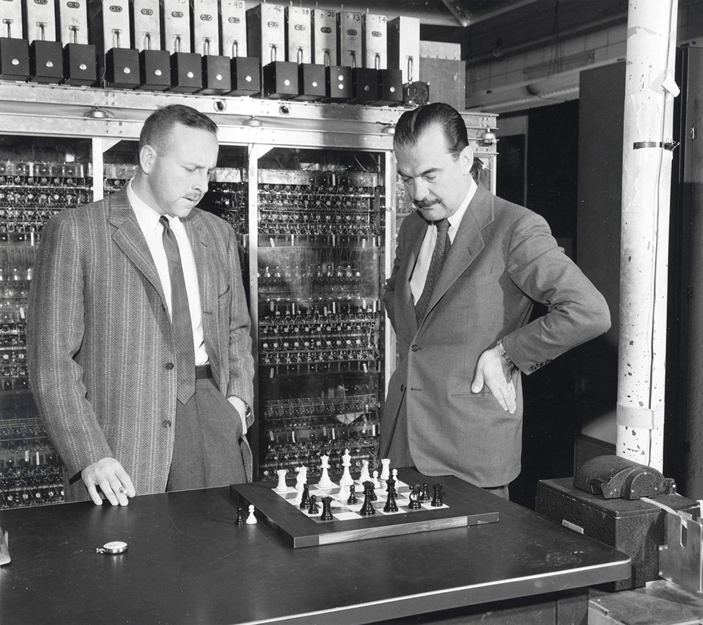
On the right is the first coauthor of the Metropolis algorithm, Nicholas Metropolis, playing a variant of chess against the computer MANIAC I at the Los Alamos Scientific Laboratory in the 1950s.

MANIAC ran the first computer aided computation of the Metropolis algorithm.

It was also the first computer to beat a human at a game of (simplified) chess in 1953. The chess was called anti-clerical chess because there were no bishops!

Nicholas Metropolis playing anti-clerical chess against MANIAC I

Metropolis-Hastings

In 1970, Wilfred Hastings extended the Metropolis algorithm to handle asymmetrical proposal distributions. This generalised algorithm became known as the Metropolis-Hastings algorithm.